Simple machine
Running the example
The complete example and the input files can be downloaded by:
git clone https://gitlab.cern.ch/lbojtar/simpa.git
The simpa/examples directory contains the script files and a directory with the input files called input_files.
To run the example code:
- Open a terminal and go to
cd simpa/examples/simple/ - Create a working directory and enter into
mkdir wdir;cd wdir - Copy the the input files needed by the SIMPA scripts
cp ../input_files/* . - Run the SIMPA CLI from the working directory (wdir). This can either be done by using the path to the jar, e.g.
java -Xmx14g -jar /your_install_dir/simpa-acc/lib/app/acc-VERSION-exe.jaror by the native launcher/your_install_dir/simpa-acc/bin/simpa-acc - The native launcher has a preset heap size of 8GB. If you need more than that, use the java command with the -Xmx option
- When the application has started, use the
call -f "../SIMPLE_MACHINE_ALL.simpa"command to run the example.
The explanation for the code in this example can be found below in the “Creating a simple machine” section.
Creating a simple machine
This example goes over the steps to construct a simple accelerator ring with six bending magnets. Please note that this tutorial will not go over all the commands and arguments for the commands, for the complete command reference, visit the Command Reference
Creating a bending magnet
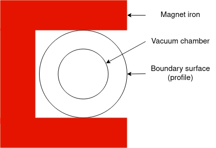
In SIMPA we reproduce the input field at a boundary surface surrounding the beam region. First, we need to create a surface around the beam region. This is done by extruding a profile along a given path. A copy of the given profile will be placed at each point of the path. The number of points in the path determines the density of the discretization of the boundary surface in the transverse direction and the number of points in the path determines the longitudinal resolution.
The boundary surface should be as far away from the beam region as possible, but it should not touch the magnet iron. The further the point sources are from the boundary surface, the smoother the field which reproduces your input field. However, you can’t place them arbitrarily far, because when we calculate their strength by a system of linear equations, the matrix might become ill-conditioned. As a rule of thumb, place the sources above the boundary surface by a distance that is about the same as the distance of grid points on the surface. This elevation must be given by the option -e in the create-tiling-config command.
following command constructs a profile with a width of 15 centimeters (7.5 right and left of the reference orbit) and a height of 6 centimeters. The x and y steps determine the density of grid points on the surface together with the longitudinal density given by the path which is used to extrude the profile.
rectprofile=create-rect-profile -xmin -0.075 -xmax 0.075 -ymin -0.03 -ymax 0.03 -xsteps 9 -ysteps 4
Then use the profile that was just created to construct the tiling configuration of the bending magnet. This command gets a flag for the name of the element (-n), the length unit used in the input file (-lu), the elevation of the sources (-e), the scaling factor for the current (-s) and the field type (-ft) which is set to static magnetic (sm)
NOTE: The element name will be used to read path points from a file called **element name**-PATH.txt
conf=create-tiling-config -n "ELBHZ" --profile rectprofile -lu "mm" -e 0.025 -s -272.995 -ft "sm"
Next, create the magnet with the tiling config created above and the allowed relative error (-re). The relative error is for the iterative solver.
create-acc-element -tc conf -re 1E-6 --solver "slice" --slice-width 1 --slice-overlap 1
The options
-solver "slice" --slice-width 1 --slice-overlap 1 are used by the slice pre-conditioner during the iterative solving.
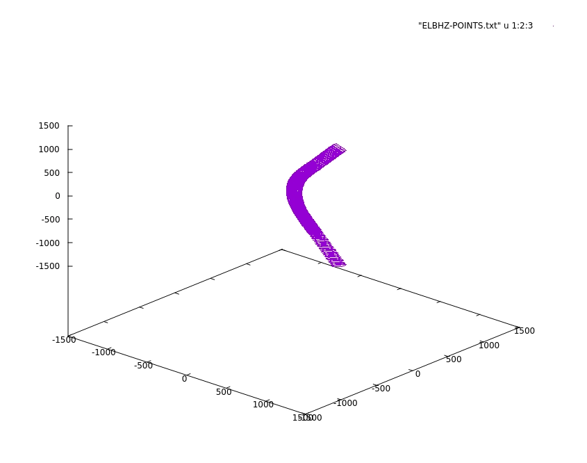
The above command will create a file called “ELBHZ-POINTS.txt”, the file can be displayed in Gnuplot by using the following command: If you plot with gnuplot use a different terminal window, otherwise you have to exit the SIMPA CLI and will loose it’s state. This is also the case for plots later !
|
A checkpoint file can be created to verify the field using the check-field command. The command below generates a file called “ELBHZ-CHECK-POINTS.txt”. We use a fixed set of file naming conventions to keep some order in the input and output files generated by SIMPA. Many commands take only the name of the element and automatically construct the file names from the name according to the conventions.
create-checkpoint-file --tiling-config conf -rss 0.002
The file “ELBHZ-CHECK-POINTS.txt” generated by the command above can be used as an input to an electromagnetic modeling software like OPERA to extract field values at those points. The location points and the field values at those locations is placed into a file according to the file naming conventions, in this case, called “ELBHZ-FIELD-AT-CHECK-POINTS.txt”. The next command calculates the relative error between the field at the checkpoints and the field evaluated by summing the point sources corresponding to this element. Some difference is expected, because the field values from OPERA, for example, are interpolated values and there is no interpolation that satisfies the Maxwell equations between 3D grid points, on the other hand, the field from the point sources satisfies them to machine precision everywhere. The point sources are scaled such that they produce the field of the magnet with 1A current, so when checking against the OPERA model we need to specify the current which was used in OPERA with the -s option, this is the same value we gave in the create-tiling-config command.
check-field --tiling-config conf
In the Opera model the X direction points inside the machine, we need to flip over so it points outside. This may or may not be needed in other cases.
xvector=create-vector3d -x 1 -y 0 -z 0
zvector=create-vector3d -x 0 -y 0 -z 1
mxvector=create-vector3d -x -1 -y 0 -z 0
bendingRot= create-rotation -v1 xvector -v2 zvector -v3 mxvector -v4 zvector
The “ELBHZ-SOLUTION.txt” will be overwritten and makes a backup ( .original)
transform-acc-element --name "ELBHZ" --rotation bendingRot
Creating the machine
After constructing the bending magnet the machine is constructed by create_sequence.simpa script file
First, add some variables for the file names (easier to change if needed).
ORBIT_FILE="orbit_design.txt"
SINGLE_ROW_COVER_FILE="SINGLE_ROW_COVER.txt"
Next, a sequence is created and selected
create-sequence --name "simplemachine"
Now it is possible to add the bendings to the sequence using the add-bending command. The flags are the name (-n), the longitudinal position in meters (-lp), the length of the magnet (-l), the name of the magnet element that should be placed (-etn), the group the bendings should be added to (-gn) and the deflection angle (-d).
add-bending -n "LNR.MBHEK.0135" -lp 4.98462 -l 0.9708 -etn "ELBHZ" -gn "BENDINGS" -d 1.0471975333
add-bending -n "LNR.MBHEK.0245" -lp 9.85102 -l 0.9708 -etn "ELBHZ" -gn "BENDINGS" -d 1.0471975333
add-bending -n "LNR.MBHEK.0335" -lp 14.71742 -l 0.9708 -etn "ELBHZ" -gn "BENDINGS" -d 1.0471975333
add-bending -n "LNR.MBHEK.0470" -lp 20.18742 -l 0.9708 -etn "ELBHZ" -gn "BENDINGS" -d 1.0471975333
add-bending -n "LNR.MBHEK.0560" -lp 25.05382 -l 0.9708 -etn "ELBHZ" -gn "BENDINGS" -d 1.0471975333
add-bending -n "LNR.MBHEK.0640" -lp 29.92022 -l 0.9708 -etn "ELBHZ" -gn "BENDINGS" -d 1.0471975333
After all the elements have been added the sequence can be closed and the reference orbit file written to a file using the end-sequence command with the -o flag specifying the reference orbit file.
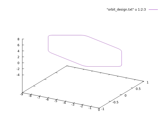
end-sequence -o ORBIT_FILE
The orbit file can be displayed in Gnuplot by using the
WARNING: Gnuplot has a bug and depending on the orientation of the plot it switches from a right-handed to a left-handed coordinate system which may make it look like the orbit was constructed counter-clockwise. Also when you plot in 2D the clockwise orbit looks anti-clockwise. |
Write the sources in the sequence to a file to check the sequence.
sequence-sources-to-file -f "allSources.txt"
The following GNUPLOT command can be used to verify if the sequence looks correct.
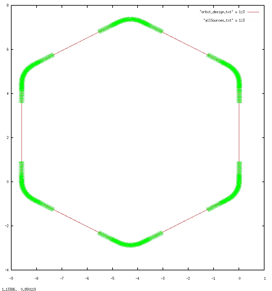 |
Creating and checking field maps
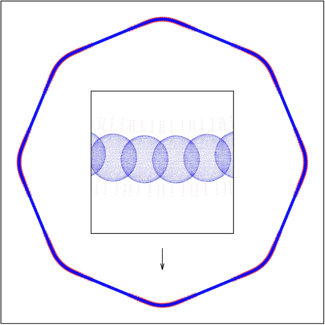
Create the cover for the orbit and write it to the file. For this command specify the aperture radius (-ar), ball radius (-br), and an output filename (-o). This cover will consist of points in a single row along the orbit. These are the center points of the covering balls that will be used to cover the beam region.
create-single-row-cover -ar 0.03 -br 0.04 -o SINGLE_ROW_COVER_FILE
Illustration of a single-row ball covering. The red dots are the point sources and the blu ones are the quadratura points on the surface of the covering spheres. During the solid harmonics expansion, the field of each point source is evaluated on each quadratura point by the Fast Multipole Method.
|
Next, expand the potentials of the magnet group (-g) with solid harmonics balls of a given degree (-l), please note that the degree has to be the same in all groups throughout the machine. In this example, there is only one group, which is the bending magnets. The following command starts the solid harmonics expansion using the file that was created at the last step (-cf). The (-re) option specifies the relative error of the SH expansion. Solid harmonic coefficients will be dropped below this limit, making the field map faster and smaller.
expand-single-row -cf SINGLE_ROW_COVER_FILE -g "BENDINGS" -l 38 -re 1e-12 -st true
The solid harmonics expansion can take a few minutes, depending on your computer speed. When it is finished a field map is created with the group name and the maximum degree of the expansion, in this case, “BENDINGS_38.bin”.
The next step is to create a scaling map to scale accelerator element groups. In this example, we have only one magnet group, but in a real accelerator, there are many. The field maps are scaled with unity, 1A current for magnetic elements, so you need to scale them according to the settings you want to make the tracking. This command creates the map.
set-scalings -m [{"BENDINGS_38.bin":-37.538}]
You need to populate the map with group names as a key and scaling factors as a value. Specify a scaling factor to the given accelerator group in the file, usually *GROUP*_*LMAX*.bin which was made with the solid harmonics expansion.
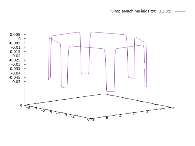
Next generate a file to check the B field of the machine, using the potential provider (-pp), a path inside the beam region, in this example the orbit design file (-f), the output length unit (-lu), and the output filename (-o).
field-on-curve -o "SimpleMachineFields.txt"
The output file can be displayed using Gnuplot with the command:
This plot displays the B fields throughout the machine. |
Tracking particles
Next, create a particle to be tracked:
pbar = create-particle --type "antiproton" -m 0.0137 -dx 0.001 -ax 0 -dy 0.001 -ay 0 -lp 2.4296 --dpop -0.0015 --name "singlerow_test_p"
To track the particle just created with the command above, the omega for Tao’s symplectic integrator must be set. This omega is a special parameter of the explicit symplectic integrator. Its value is in the range of 0.. 2*Pi. It is used to make the integrator stable and minimize the energy oscillations. It is not very sensitive, usually in a few tries, one can find a good enough value. If it’s very far off, the particle will be lost in a few turns or less. This is a bit of an annoyance when running the tracking for the first time, specially if it is not clear if the particle was lost because the field scaling is wrong or the omega parameter is far off.
set-integrator -om 2.5
track --particle pbar --turns 1000 --step-size 0.01 -dr 0.1
The command above adds a phase space observer automatically at position zero to the tracker to print and generate output during the tracking. It will construct a disk at the longitudinal position zero (can be changed with the -phop option) with the given disk radius (-dr option). This observer will write the phase space coordinates to a file whenever the particle passes through the disk. The disk radius should be big enough to cover the aperture, but not too big, otherwise, it may intersect the beam region twice.
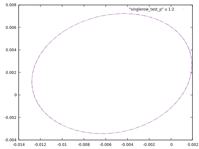
The track command will output the file “single_row-PHS-AT_0.000.txt” according to the particle name, which can be displayed in Gnuplot with the command:
The output of this command should look like the following image:
This plot displays the X and Y location of the particle when it passes through the phase-space observer. |